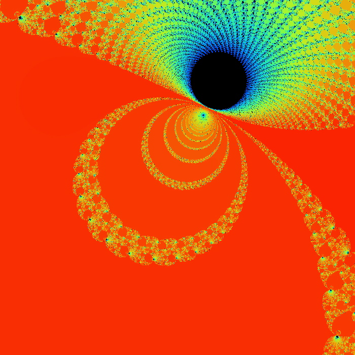
Distributed Mandelbrot Set Generator

Motivation

Inspired by my general fascination with parallel and distributed methods of computation, and subsequently triggered by a course I took in parallel algorithms, I decided to implement a distributed processor to perform time-intensive computations. I chose to do this from the ground up rather than using conventional packages for distributing processing jobs over a network of computers, primarily because that was the fun part. I didn't really care about getting the computations done. In fact I had to search for a candidate problem to solve. I wanted to learn how to implement a client-server system for sending out pieces of a job and then arranging the pieces as they come back.

The Problem

So what problem did I pick? Distributed networks of processors require a high processor-work to network-traffic ratio. Unlike a parallel processing machine, passing messages between the processors is extremely expensive (slow), and since there is no shared memory, I needed a problem where small amounts of data transferred over the network could spawn larger quantites of computation. Equally helpful would be a problem where the distributed jobs didn't need to communicate with each other in order to perform their computations.

Fractals are a perfect solution. Any one part of the image (say one pixel) is totally independent from all other parts of the image, so the image can literally be chopped up into pieces and the pieces can be sent out to different processors. When a particular section of the image is calculated, the corresponding bitmap can be sent back to the server, which can arrange the sections as they arrive. Actually, what I just said isn't absolutely true. There can be a correlation between a given pixel's value and the values of nearby pixels, so heuristic methods can probably be devised that reason about the image with a semblance of intelligence. However, it remains true that any one pixel can be calculated without taking into account any other pixels in the image.

The Setup

So fractals: I chose the mandelbrot set purely for it's wide recognition. My system consists of a server (a 233 MHz G3 imac with 64 megs of RAM running MacOS 8.6.1 ) and any available computer on the internet as a potential client (although I only wrote client software for a standard Linux or Unix box). I used the "gig" machines in the computer science department at the University of New Mexico. There are 10 gig machines, each of which has a dual 450 MHz Pentium III with 1 gig of RAM running Debian 2.2 Linux. The server has a GUI that lets the user navigate the mandelbrot set with ease. A given image can be generated either on the server alone (which I did on my own 500 MHz G3 Powerbook with 256 megs of RAM running MacOS 9.0.4) or can be sent out to the clients, each job's bitmap being accepted back in arbitrary order and its section of the image being drawn on the screen as it is sent back. The number of potential clients is essentially unbounded.

The Images

There are graphs below showing data on the performance of the system I set up. I collected data on the generation of four images from within the mandelbrot set. These images were selected to cover a range of circumstances in fractal images. The images on this page are 150 pixels square. However, the images that were actually generated by the system were 700 pixels square. Click on the images on this page to see the full-size images that were generated. The images are 8-bit, one byte per pixel, which makes it easy to calculate the size of a given image based on its dimensions.

Left edge (real): 0.2500590408486983 Top edge (imag): -0.0000007818639277 Resolution: 0.0000000000745058 Max iterations: 16384 Total iterations: 305,764,434	Left edge (real): 0.2515137590680807 Top edge (imag): -0.4985213797433037 Resolution: 0.0000003051757813 Max iterations: 8192 Total iterations: 387,995,302	Left edge (real): -1.9537137262834396 Top edge (imag): 0.0000839115943448 Resolution: 0.0000000000000023 Max iterations: 4096 Total iterations: 71,620,611	Left edge (real): -1.0592561124052318 Top edge (imag): -0.2634518454756054 Resolution: 0.0000000000000023 Max iterations: 512 Total iterations: 33,400,876
Each image is divided into horizontal stripes that will be distributed amongst the clients. This image is extremely unbalanced, requiring much heavier calculation at the top than the bottom. It is also an overall heavy image with over 300,000,000 iterations of the inner loop of the mandelbrot set algorithm.	This image is pretty balanced, although a little heavier toward the top and bottom. It is, however, the heaviest calculation in the set with over 380,000,000 iterations.	This image is unbalanced, heavy toward the center, but it is a relatively thin image overall with barely 70,000,000 iterations.	This image is extremely balanced and also very thin on the overall calculation with only a little more than 30,000,000 iterations.

Load Balancing Methods

I experimented with three different methods of load balancing. The first method divides the number of rows (700 you will recall) amongst the processors in proportion to each processor's individual performance either on a test that the client runs before logging into the server or based on the client's performance on the previous image.

The second method consists of the server generating an image with one percent the area of the primary image (70x70 pixels). The server then weights each row based on the number of iterations required to generate that row. All 700 rows in the primary image are then interpolated from the 70 row weights in the small image. The rows are then divided evenly amongst the clients based on their weights.

The third method is simply an overlap of the first two methods. Since the first two methods are orthogonal to each other, it is easy to apply, one, the other, or both methods.

For comparison purposes, I also tested the system with no load balancing by simply dividing the number of rows evenly amongst the processors.

The Data

I generated each of the four images 41 times with different settings. One of these settings was without the server-client distribution, simply generating the image on a 500 MHz Powerbook (a mac). The other 40 times consist of four load-balancing methods (including no balancing at all) crossed with one client up through ten clients. It should be bared in mind that although the clients are essentially equivalent computers, their performance was not. Due to the load on each individual machine when I generated the images, the calculation speed of the clients differed by a factor of two. That is, the fastest clients were running twice as fast as the slowest clients, with the average speed resting somewhere about two thirds of the way from the slowest to the fastest client.

I generated three graphs for each image. The first graph shows the generation time for the image.

The second graph basically shows the same data as the first graph, but from a different perspective: the calculation rate of the system as a whole, measured in iterations per second.

The third graph shows the efficiency of the system as a whole. I measured efficiency as a ratio of the time the client-processors were calculating to the overall time of the image generation. For example, assume two clients are working on an image. Client A works on its section of the image for one time unit before finishing its calculation and returning its associated bitmap to the server. Client B works on its section of the image for two time units. The total amount of time spent working is three time units, but the total amount of time that client processors were tied up is four time units, so the efficiency is 75 percent. Obviously, it's easy to see that if all the clients return their image sections as the same time, the efficiency will be 100 percent.

The Graphs

The first thing to make a note of is the fact that the ten gig machines were working at various speeds (I believe due to process load, not hardware differences) when I accumulated the data. Some of the machines were as much as twice as fast as other machines. This produces bizarre results. For example, in this first image load balancing with image prediction performed worse with two processors than with one. This is because the second processor was running so slow that it was just getting in the first processor's way. The image prediction method of load balancing doesn't take into account differences in processor speed. The reason that two processors with no load balancing did all right is that the second (slow) processor got the lower half of the image (just by luck), which accounts for considerably less than half the necessary computation. Notice that overall, green beats red, which means predicting the image has more effect than evening out the processing power (on this particular image). However, combining both methods blows all the other methods away. Look at the efficiency for the combined method. It never dips below 90 percent.

This image is much more vertically uniform than the first image. As a result the image prediction method has little effect on the performance. The minor differences between the green and the black lines are primarily due to the image being chopped up differently and slightly larger or smaller than average sections going to the faster or slower processors just by chance. Notice that both methods which employ processor-speed balancing do show improvement however, for obvious reasons. A good point to make after seeing the first two graphs is that if the image is unbalanced, then predicting and distributing the image evenly pays off more than distributing the image in sections of size proportional to the clients' processing speed. If the image is balanced however, then image prediction will have very little effect and thus is basically the same as no load balancing at all. So at that point it is beneficial to balance based on processor speed. It seems pretty obvious, however, that if the range in processing speeds were much greater than the factor of two exhibited here, that the processor-speed balancing method would pay off much more in that case.

This is another image that in unevenly balanced from row to row, so the methods that predict row weight ahead of time have a noticable payoff. However, although the green line is unquestionably better than the black and red lines, it is only slightly better. The addition of processor-speed balancing to the image prediction method makes a phenomenal difference. This is because the center of this image is so much heavier than the periphery that without balancing the processor-speeds, processors working on the top and bottom are virtually guarranteed to end up wasting lots of time, even with image prediction running.

This image is extremely balanced and the graphs show this well. There is a sharp divergence between the performance of methods that employ processor-speed balancing and those that don't. Image prediction balancing has absolutely no effect either alone or in combination since the image prediction just divides up the image evenly, which is exactly what the no-balancing-of-any-kind method is doing in the first place. I will reiterate that client number two was running at less than half the speed of client number one so data at position two always looks a little peculiar as a result. In all four images, dividing the actual calculation in two (using the image prediction method) hurts the system as a whole terribly because slow client two is doing the same amount of work as fast client one. Once again, the reason the running time actually drops from two clients to one is that client one was running more than twice as fast as client two and so it could do the whole job faster on its own. Obviously, when using the load balancing methods that take this fact into account, the performance once again improves with two clients, as would be expected.

Discussion

The first conclusion I came to as a result of this project was that macs rule!!! My 500 MHz G3 mac averages somewhere around 14.5 to 15 million iterations per second while the fastest clients (dual 450 Pentium IIIs) averaged about 2.5 million iterations per second. Now 15 divided by 2.5 is 6, but it's obvious from the graphs that the mac actually holds its own up to about a 7.5 processor system. The reason for this is that although the fastest clients were running about 2.5 million iterations per second, the slowest clients were running closer to 1.2 million iterations per second. The average of those values is 1.85 and 14.5 divided by 1.85 is right around 7.8.

Enough about the mac. What else is there? Well, I think the thing that stands out most when I look at the graphs is how the efficiency changes depending on the method of load-balancing being used. Yeah, all the graphs show improvement with various forms of load-balancing, but with the maximum load-balancing employed (both processor-speed balancing and image prediction) the efficiency never drops below 90 percent and appears to average higher than 95 percent. That's truly remarkable. That means the distributed system as a whole is performing virtually as well as it could possibly hope to perform under even the most ideal circumstances, and just in case you're wondering, yes the time for the job to complete when using image prediction does include the time it takes the server to generate the one percent small image and weight the rows accordingly. In fact, all the times include all related overhead such as dividing up the job by whatever means is chosen between the clients. This sort of stuff tends to be utterly neglibable however.

A fairer concern is how much of the time is being spent just shuffling data around the network. To send a job to a client requires barely 100 bytes of data. The server simply sends a few coordinates in the complex coordinate plane telling the client where its rectange is (its slice of the image), how far to iterate the mandelbrot set algorithm, etc. To get the image back is a little more daunting however. I was producing 8 bit images, so a 700x700 image is 490,000 bytes, just shy of half a meg. Now, any one client won't be sending back that much data (except in the case of a single client system which I did include in my data and on the graphs), but regardless of how much data each client must send, the server must be capable of accepting a half meg of bitmap data fairly quickly. If the clients all report back simultaneously, the server may be receiving a consider amount of data all at once. In fact, given an efficiency of 100 percent, the necessary incoming bandwidth of the server approaches infinity as the number of clients increases. Imagine 490,000 clients, each working on one pixel, all send back the bitmap of that pixel at the same moment. The server wouldn't be receiving a stream of 490,000 bytes; it would receive 490,000 bytes simultaneously. As it turns out, over ethernet even a half meg of data doesn't put much of a dent into the elapsed time. I didn't specifically measure the amount of time spent transferring data, but the GUI I designed shows me what stage of the process each client is in: waiting-for-a-job, working-on-a-job, sending-a-job-bitmap-back, or done-working-on-a-job and waiting for the other clients to finish. The last state consitutes wasted time incidently, which counts against efficiency. Well, my point is that the state of the clients would generally flash from working to done-working so fast that I didn't even see the intervening job-returning message. That's how fast the bitmaps came back.

Future Work

I'm basically done with this project, but I do have some ideas. One thing is that I believe heuristic algorithms could be designed that would cut down the time required to calculate an entire image. For example, areas where the mandbelrot set algorithm maxes out of iterations tend to clump together. I believe, although I haven't proven this rigorously, that any closed perimeter of such pixels in any arbitrary shape is guaranteed to be filled with maxed out pixels that don't need to be calculated at all. This would be of great benefit because it is precisely the maxed out areas that cost so much to calculate because each individual pixel takes the maximum number of iterations to calculate.

As for ideas that could be applied to the distributed network, I'm ready to move on. Now that I know how to set up a distributed network of processors, I don't care about fractals anymore. They were just a means to an end. What I would really like to do is set up a massive artificial life simulation (the details of which I am vague about because I have only a vague notion of this idea). To help aid the requirement that most computation occur within and not between processors, each client machine could house a "world' and the alife agents could be confined to interacting with other agents in that world. The agents could choose to traverse the network from one world to another, but there wouldn't be too much direct interaction between the worlds. Think of isolated islands or planets or something like that. This alife system I'm dreaming up isn't really a client-server system. It's more like Gnutella than Napster to borrow a readily recognized example.

Of course, while I'm busy designing this thing in my head, I'm also thinking it would be cool if human users could jump in and interact with the system too. Now this is starting to sound like a distributed networked mud of some sort. Viva la Internet! Viva! Viva!

If you have any thoughts on this project, please feel free to email me. I would love to hear what people think.